Contents
Warning
I'm sharing this code, a byproduct of my university assignment, with a healthy dose of trepidation. Let's face it, it's probably a hot mess, but I'd be eternally grateful for your feedback. I'm still navigating the complexities of different models, so keep in mind that what you're about to read might be riddled with inaccuracies or just plain wrong. Any correction is welcomed.
My codebase is a work in progress (read: bug-ridden) and I'd love your feedback to help me level up my coding skills.
The Fundamentals
A Boltzmann Machine is a model of pairwise interacting units where each unit updates its state over time in a probabilistic way depending on the states of the neighboring units[1]. Or, in other words, is a neural network of units whose activation is determined by a stochastic function. The network includes both visible (data) v and hidden (latent) h units. It learns a probability distribution from the training data, but training the parameters of the BM model is computationally intensive. To reduce the complexity, the connectivity of the BM is restricted.
The Restricted Boltzmann Machine (RBM) is a type of probabilistic graphical model that serves as a fundamental component in the construction of deep belief networks (DBNs). Additionally, RBMs are widely recognized as effective density models, capable of extracting meaningful features from complex data sets[2].
RBM
More formally, a Restricted Boltzmann Machine is a particular type of Markov random field that has a two-layer architecture, that forms a bipartite graph, i.e. there are connections only between hidden and visible units. The visible stochastic units v are connected to hidden stochastic units h
. The probability of the joint configuration {v, h} is given by:
Where is the normalizing constant and
are the model parameters, with W representing visible-to-hidden symmetric interaction terms, and
representing visible and hidden biases respectively.
Learning becomes tractable due to graph bi-partition which factorize the distribution. The crucial assumption here is that the hidden units are conditionally independent given the visible units, and vice versa. In other words, once we know the values of the visible units, the hidden units become independent of each other, and similarly, once we know the values of the hidden units, the visible units become independent of each other. This assumption allows us to simplify the inference and learning processes, in formula:
By updating these parameters in batches, we can process multiple data points or samples together, which can reduce the overall computational cost and speed up the learning process.
Training RBM
A joint configuration, (v, h) of the visible and hidden units has an energy given by:
The network assigns a probability to every possible pair of a visible and a hidden vector via this energy function:
Where the normalization term is given by summing over all possible pairs of visible and hidden vectors:
The probability that the network assigns to a visible vector, v, is given by summing over all possible hidden vectors:
Given independent and identically distributed (i.i.d) variables to learn the RBM we use the maximum likelihood estimator:
The derivative of the log probability of a training vector with respect to a weight is simple:
where denotes an expectation with respect to the data distribution:
and is an expectation with respect to the distribution defined by the model,
. Exact maximum likelihood learning in this model is intractable because the computation of the log loss function is exponential in the number of visible or hidden units. Instead, learning can be performed by following an approximation to the gradient by Gibbs sampling. To approximate
we can: clamp the data to obtain something that is binary (continuous[4]). Sample
for all pairs of connected units. Repeat for all elements of dataset. To sample
we can: let the network reach equilibrium by sampling
for all pairs of connected units. Repeat many times to get a good estimate (infinity for the best result).
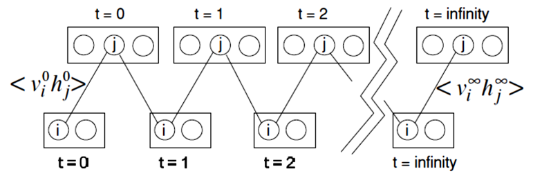
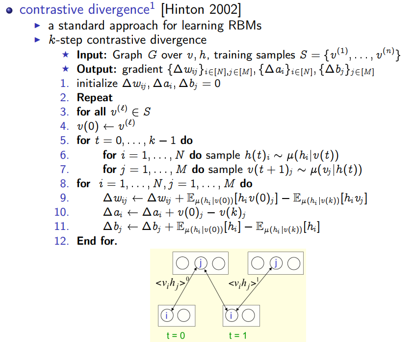
Gibbs sampling can be painfully slow to converge, thus usually Contrastive Divergence [6] is used. In a nutshell, Contrastive Divergence (CD) is a popular machine learning algorithm that in theory does not follow the gradient of any function, but in practice works. CD iterates between generating samples from the current model and using these samples to estimate the gradient of the log-likelihood function. This gradient estimate is then employed to optimize the model parameters, enabling CD to effectively learn Deep Belief Networks.
Complete algorithm:
My Implementation
Warning: Proceed with caution: this code might be wrong. Please, let me know if you find any errors.
For your convenience, I've made the resource available in my public Google Colab notebook, where you can access and explore the code, data, and results. link
To evaluate my RBM implementation, I'm training it on the MNIST training set and encoding the test set in the hidden units vector for each image. I then split the encoded data into two parts: one for training multiple classifiers and another for evaluating their performance on unseen data.
Setup and Download the dataset
import gzip
import os
from urllib.request import urlretrieve

train_img_url = "http://yann.lecun.com/exdb/mnist/train-images-idx3-ubyte.gz"
train_label_url = "http://yann.lecun.com/exdb/mnist/train-labels-idx1-ubyte.gz"

current_dir = os.getcwd()
train_imgs_name_f = 'train_imgs.gz'
label_imgs_name_f = 'train_labels.gz'
train_img_path = None
train_label_path = None

def check_or_download(url, file_name):
    path = None
    if not os.path.exists(file_name):
        path, _ = urlretrieve(url, file_name)
        print(f"Downloaded {file_name}")
    else:
        pwd = os.getcwd()
        path = os.path.abspath(f"{pwd}/{file_name}")
        print(f"{file_name} already exists")
    return path

path_imgs = check_or_download(train_img_url, train_imgs_name_f)
path_labels = check_or_download(train_label_url, label_imgs_name_f)

with gzip.open(path_imgs, 'rb') as train_imgs_f:
    train_imgs = train_imgs_f.read()

with gzip.open(path_labels, 'rb') as train_labels_f:
    train_labels = train_labels_f.read()
Read the dataset to the memory
import matplotlib.pyplot as plt
import numpy as np
import tqdm

image_size = 28
num_images = 60000

data = np.frombuffer(train_imgs, dtype=np.uint8, count=image_size*image_size*num_images, offset=16).astype(np.float32)
data = data.reshape(num_images, image_size, image_size, 1)

Image Binary Encoding
I employed random clamping to convert the data into a binary vector.
numpy_rng = np.random.RandomState(89377)
data /= 255

rand_d = numpy_rng.rand(*data.shape)

data = (rand_d < data).astype(np.float32)
Initialization of the visible bias
len_v_vec = data.shape[1] * data.shape[2]
def getVbias(dataset):
    data = dataset.reshape(dataset.shape[0], len_v_vec)
    p = np.count_nonzero(data, axis=0)/data.shape[0]
    p = p/(1-p)
    p[p == 0] = 1.0
    return np.log(p)

bias_visible = getVbias(data)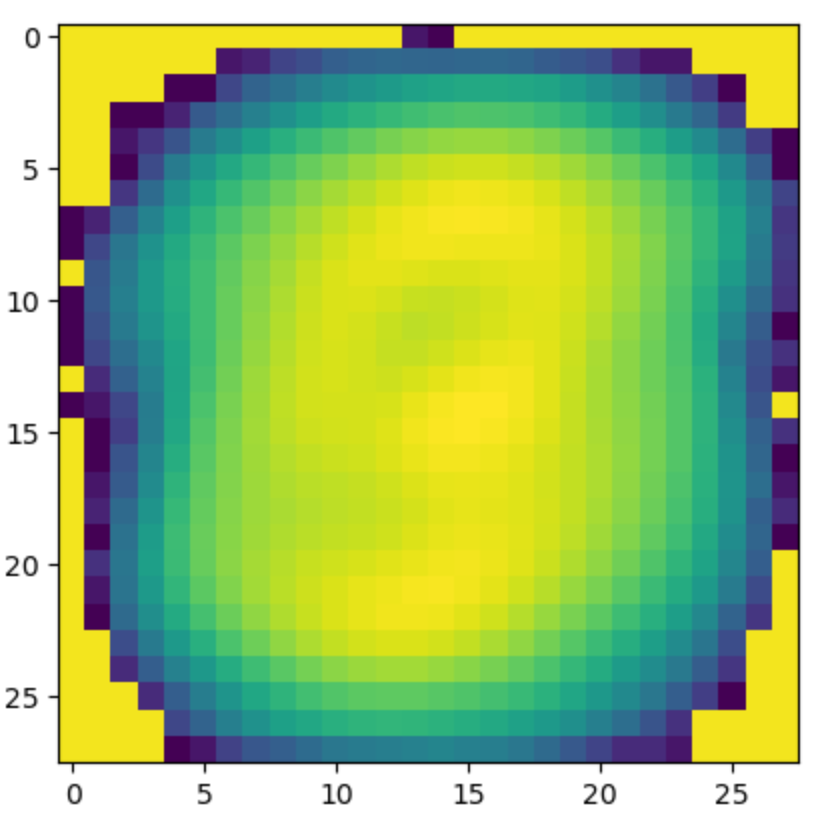
The Implementation of the Restricted Boltzmann Machine
The weights are initialized by drawing random samples from a normal distribution with μ(x) = 0 and σ(x) = 0.01
class Trainable():

    def __init__(self, num_row, num_column) -> None:
        self.weights = numpy_rng.normal(loc=0.0, scale=0.01, size=(num_row, num_column))
        self.prev_gw = np.zeros(self.weights.shape)
        self.prev_gbv = np.zeros(num_row)
        self.prev_gbh = np.zeros(num_column)
        self.t_iter = 0
        self.prev_p_h0 = np.zeros(num_column)


    def compile(self, batch_size, epochs, learning_rate, weight_cost, momentum):
        self.batch_size = batch_size
        self.epoch_size = epochs
        self.learning_rate = learning_rate
        self.weight_cost = weight_cost
        self.momentum = momentum

        return self

    def calculate_gradient(self, data):
        pass

    def predict(self, data):
        pass

    def update_weights(self, gradient):
        self.weights += gradient['gw']
def sigmoid(x):
return 1 / (1 + np.exp(-x))
def bernoulli(p):
return (numpy_rng.rand(*p.shape) < p).astype(np.float32)
class RBM(Trainable):
def __init__(self, num_visible_units, num_hidden_units, biasV=None) -> None:
self.num_hidden_units = num_hidden_units
self.num_visible_units = num_visible_units
self.biasH = np.zeros(self.num_hidden_units) #np.random.uniform(low=-0.00001, high=0.00001, size=(self.num_hidden_units, 1)).squeeze()
self.biasV = biasV if biasV is not None else np.random.uniform(low=-1, high=1, size=(self.num_visible_units, 1)).squeeze()
super().__init__(self.num_visible_units, self.num_hidden_units)
@property
def num_visible(self):
return self.num_visible_units
@property
def num_hidden(self):
return self.num_hidden_units
def sample_hidden(self, visible_units):
activation = (visible_units @ self.weights) + self.biasH
h1_mean = sigmoid(activation)
return h1_mean, bernoulli(h1_mean)
def sample_visible(self, hidden_units):
activation = (hidden_units @ self.weights.T) + self.biasV
v1_mean = sigmoid(activation)
return v1_mean, bernoulli(v1_mean)
def get_energy(self, visible_units):
hidden_units = self.sample_hidden(visible_units)
s = visible_units.T @ self.weights @ hidden_units[1]
return ( - s - self.biasH.T @ hidden_units[1]- self.biasV.T @ visible_units).sum()
def cd_sampling(self, visible_units):
visible_units = np.zeros((1, self.num_visible_units)), visible_units
while True:
hidden_units = self.sample_hidden(visible_units[1])
yield visible_units, hidden_units
visible_units = self.sample_visible(hidden_units[1])
def update_weights(self, gradient):
return super().update_weights(gradient)
# Remember v1, h1 are tuples of (probability, sampled)
# Remember each value of key is a tuple of (v1, h1)
def predict_h1(self, data):
print(data.flatten().shape)
if data.ndim == 3:
data = data.flatten()
passes = self.cd_sampling(data)
v0, h0 = next(passes)
v1, h1 = next(passes)
print(v1)
return v1,h1
else:
data = data.reshape(data.shape[0], self.num_visible_units)
predictions = {}
for i, d in tqdm.tqdm(enumerate(data)):
passes = self.cd_sampling(d)
v0, h0 = next(passes)
v1, h1 = next(passes)
predictions.update({i: (v1, h0)})
return predictions
def train(self, data):
data = data.reshape(data.shape[0], self.num_visible_units).copy()
total_size = data.shape[0]
energy_error = []
error = []
for epoch in range(self.epoch_size):
error.append([])
energy_error.append([])
print(f"Epoch {epoch+1} out of {self.epoch_size}")
for i in tqdm.tqdm(range(0, len(data), self.batch_size)):
if i + self.batch_size > total_size:
self.batch_size = total_size - i
batched_data = data[i:i+self.batch_size]
gradient = self.calculate_gradient(batched_data)
self.update_weights(gradient)
self.biasV += gradient['gbv']
self.biasH += gradient['gbh']
energy_error[epoch].append(gradient['energy_error'])
error[epoch].append(gradient['error'])
del gradient
plt.hist(self.weights.flatten(), bins='auto')
plt.title("Histogram of Weights -- Epoch {}".format(epoch+1))
plt.show()
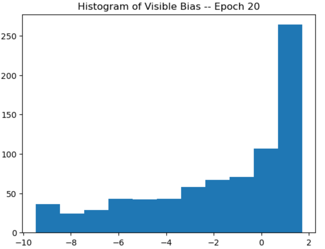
plt.hist(self.biasV, bins='auto')
plt.title("Histogram of Visible Bias -- Epoch {}".format(epoch+1))
plt.show()
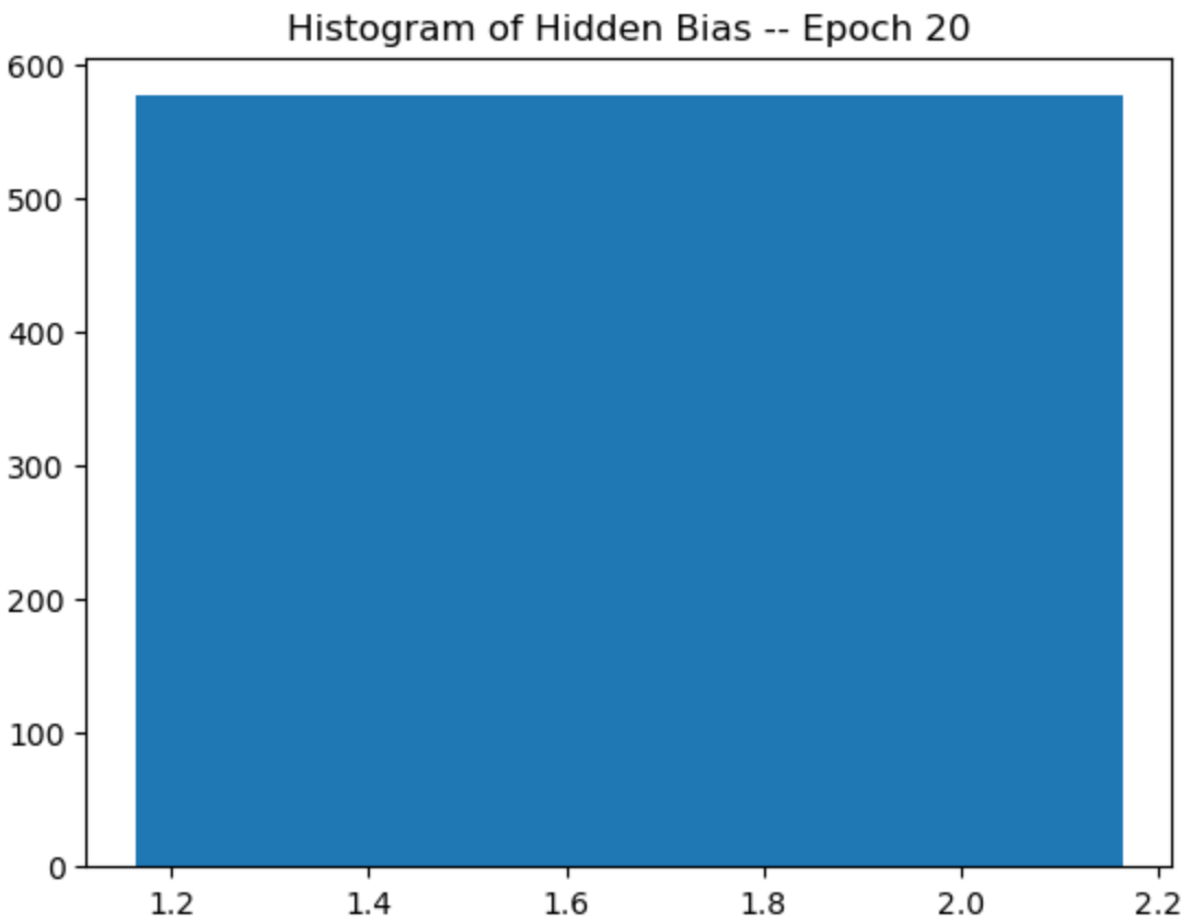
plt.hist(self.biasH, bins='auto')
plt.title("Histogram of Hidden Bias -- Epoch {}".format(epoch+1))
plt.show()
self.prev_p_h0 /= data.shape[0]
prob_img = self.prev_p_h0.reshape(24, 24)
plt.imshow(prob_img, cmap='gray')
plt.title("The Average Probability of Hidden Units of the batch")
plt.show()
self.prev_p_h0 = np.zeros(self.num_hidden_units)
if self.momentum < 0.9 and epoch == self.epoch_size // 3:
self.momentum += (0.9 - self.momentum) / (self.epoch_size / 2)
print(f"Epoch Mean Square Error {np.array(np.mean(error[epoch]))} ---- Energy Error {np.array(energy_error[epoch]).mean()}")
return self.weights, self.biasV, self.biasH, energy_error, error
def calculate_gradient(self, batched_data):
np.random.shuffle(batched_data)
updates = {"gw": np.zeros(self.weights.shape), "gbv": np.zeros(self.biasV.shape), "gbh": np.zeros(self.biasH.shape), "energy_error": 0, "error": 0}
def calc_deltas(data, updates):
passes = self.cd_sampling(data)
v0, h0 = next(passes) # v0[0] is the 0 vector of the visible units, v0[1] is the actual data
v1, h1 = next(passes) # v1[0] is the probability , v1[1] is the sampled visible units
updates['gw'] += (np.outer(v0[1].T, h0[0]) - np.outer(v1[1].T, h1[0]))
updates['gbv'] += (np.sum(v0[1]) - np.sum(v1[0]))
updates['gbh'] += (np.sum(h0[1]) - np.sum(h1[0]))
updates['error'] += np.mean((v0[1] - v1[1])**2)
self.prev_p_h0 += h0[0]
updates['energy_error'] += (self.get_energy(v0[1]) - self.get_energy(v1[1])).mean()
return data
np.apply_along_axis(calc_deltas, 1, batched_data, updates)
updates['gw'] /= self.batch_size
updates['gbv'] /= self.batch_size
updates['gbh'] /= self.batch_size
updates['gw'] = self.momentum * self.prev_gw + (1. - self.momentum) * updates['gw']
updates['gbv'] = self.momentum * self.prev_gbv + (1. - self.momentum) * updates['gbv']
updates['gbh'] = self.momentum * self.prev_gbh + (1. - self.momentum) * updates['gbh']
self.prev_gbv = updates['gbv']
self.prev_gbh = updates['gbh']
self.prev_gw = updates['gw']
updates['gw'] = self.learning_rate * (updates['gw'] - self.weight_cost * self.weights)
updates['gbv'] = self.learning_rate * updates['gbv']
updates['gbh'] = self.learning_rate * updates['gbh']
updates["energy_error"] /= self.batch_size
updates["error"] /= self.batch_size
self.prev_p_h0 /= self.batch_size
return updates
rbm = RBM(len_v_vec, 576, bias_visible)The training process updates the parameters in batches, leveraging momentum, L2 regularization, and a learning rate to optimize the model. For each piece of data, it computes the positive phase (wake) and the negative phase (dream) and accumulates the difference. Same for the visible and hidden biases. This sum is then divided by the batch size to obtain the average gradient. To improve clarity, I've chosen to calculate the update for the weight parameters as follows:
Model Training
Starts with 0.5 momentum and then increases, the maximum is 0.9. I experimented with various learning rates and weight decay values (e.g., learning rate = 0.0001, weight decay = 0.00001). However, the model's accuracy only reached 0.9. Among all the values I explored, the configuration below yielded the best results.
conf = {
    "momentum": 0.5,
    "weight_cost": 0.00008,
    "learning_rate": 0.08,
    "epochs": 20,
    "batch_size": 128,
}

rbm.compile(**conf)
r = rbm.train(data)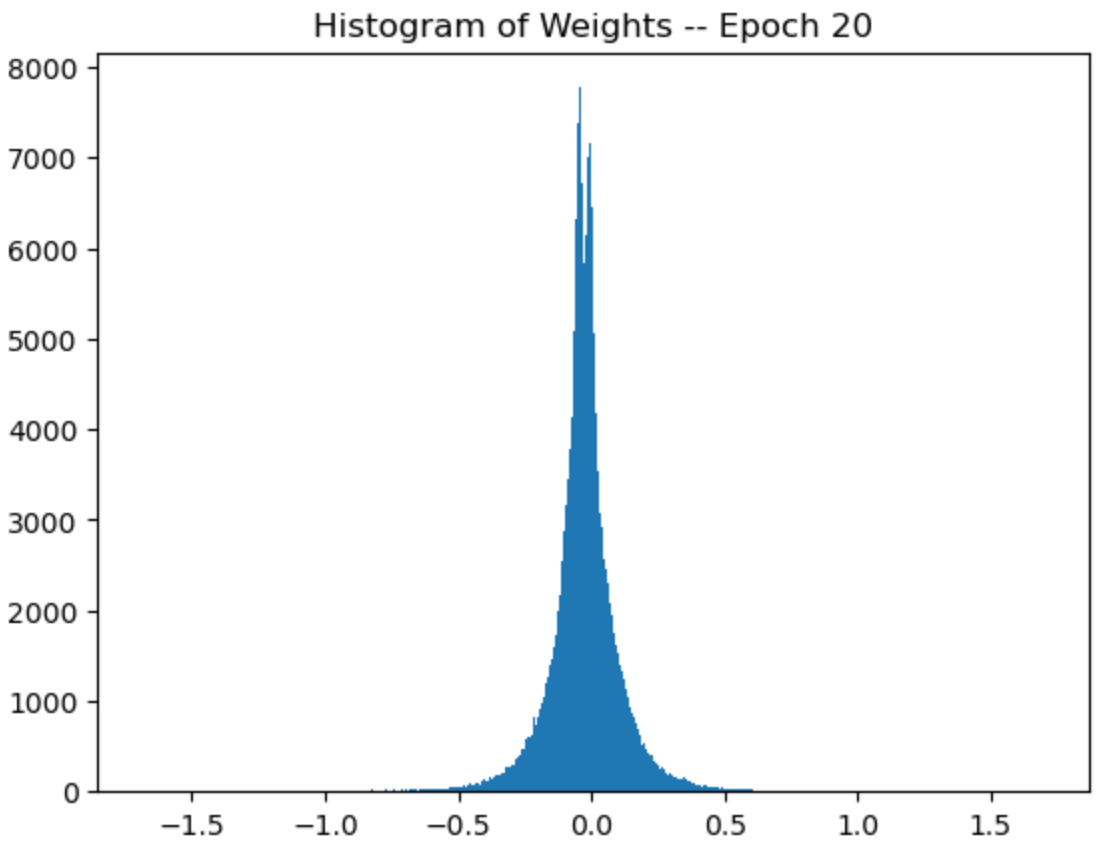

Test set download
test_url = "http://yann.lecun.com/exdb/mnist/t10k-images-idx3-ubyte.gz"
test_label_url = "http://yann.lecun.com/exdb/mnist/t10k-labels-idx1-ubyte.gz"

test_imgs_name_f = 'test_imgs.gz'
test_label_imgs_name_f = 'test_labels.gz'

path_test_imgs = check_or_download(test_url, test_imgs_name_f)
path_test_labels = check_or_download(test_label_url, test_label_imgs_name_f)

with gzip.open(path_test_imgs, 'rb') as test_imgs_f:
    test_imgs = test_imgs_f.read()

with gzip.open(path_test_labels, 'rb') as test_labels_f:
    test_labels = test_labels_f.read()
Applying same stochastic method for clamping
test_data = np.frombuffer(test_imgs, dtype=np.uint8, count=image_size*image_size*10000, offset=16).astype(np.float32)
test_data = test_data.reshape(10000, image_size, image_size, 1)
test_data_size = test_data.shape[0]


rand_d = numpy_rng.rand(*test_data.shape)


test_data = (rand_d < test_data).astype(np.float32)
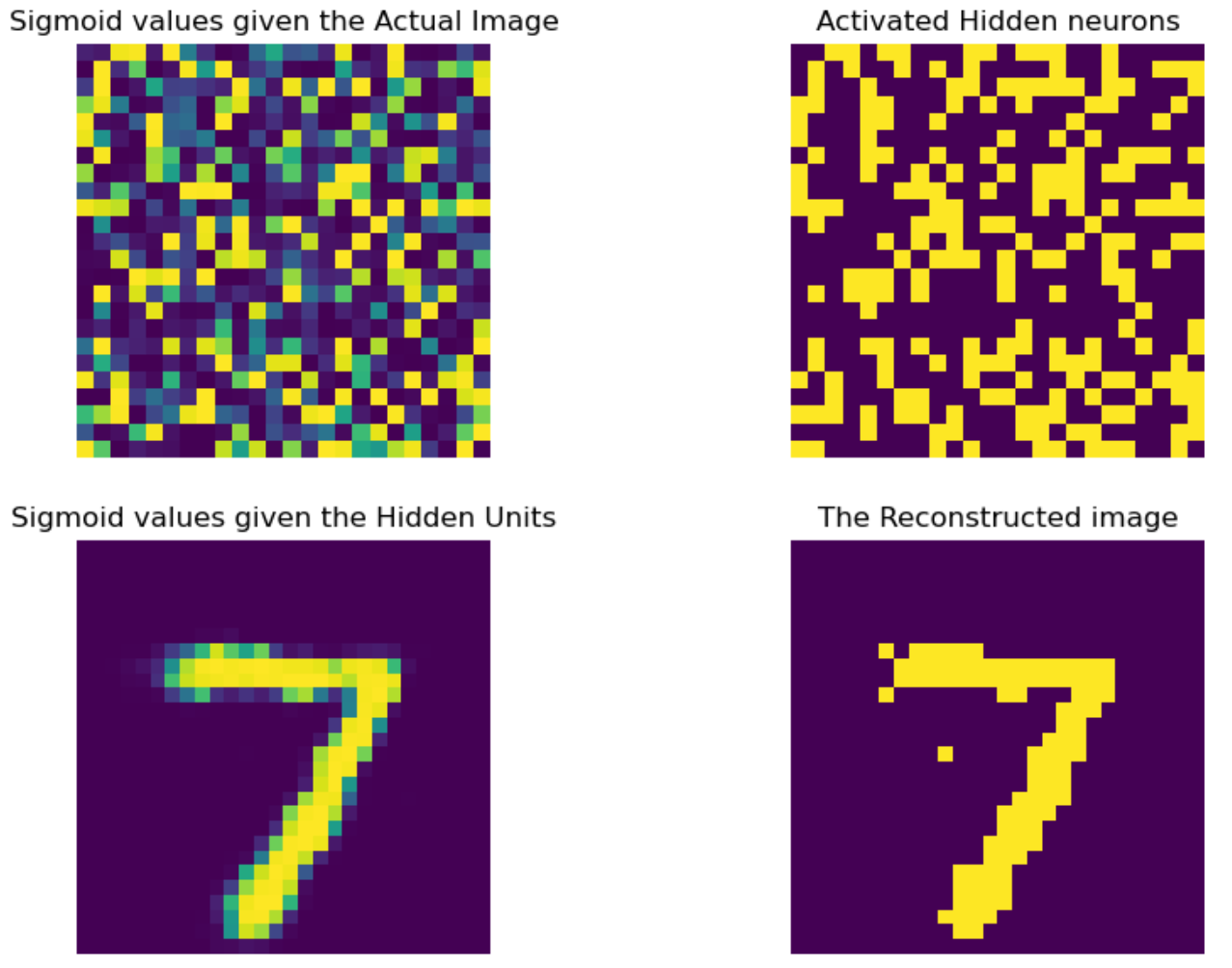
The predict_h1 method returns a dictionary. The keys are numerical, ranging from 0 to the total number of test data points. Each key corresponds to a tuple containing two elements:
v1: This is another tuple containing the sigmoid activations for the visible layer and the reconstructed images.h0: This tuple includes the sigmoid activations and the activated hidden layer neurons.
pred_test = rbm.predict_h1(test_data)
Classification
1. AdaBoostClassifier
from sklearn.model_selection import train_test_split
from sklearn.ensemble import AdaBoostClassifier
clf = AdaBoostClassifier(n_estimators=400, algorithm="SAMME", random_state=89377)
nb = clf.fit(X_train, y_train)
print(nb.score(X_test, y_test)) # 0.8212121212121212
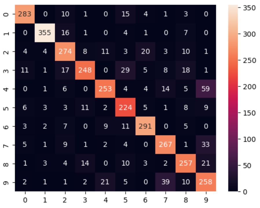
sns.heatmap(confusion_matrix(y_test, nb.predict(X_test)), annot=True, fmt='d')While AdaBoostClassifier showed some improvement in accuracy with more iterations, this approach risks overfitting according to this. Given its lower performance compared to other algorithms, it might be best to explore alternative models for better efficiency and generalizability.
2. MLPClassifier
from sklearn.neural_network import MLPClassifier
clf = MLPClassifier(hidden_layer_sizes=450, random_state=89377, activation="relu", alpha=0.0008, learning_rate="constant", learning_rate_init=0.008, max_iter=600)
nb1 = clf.fit(X_train, y_train)
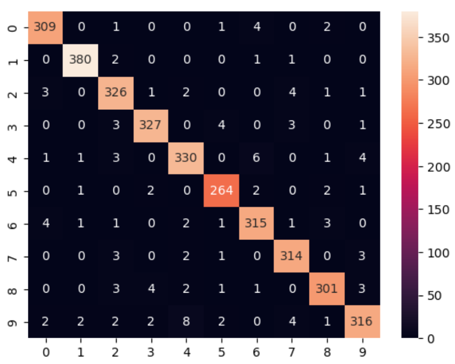
print(nb1.score(X_test, y_test)) # 0.9642424242424242
sns.heatmap(confusion_matrix(y_test, nb1.predict(X_test)), annot=True, fmt='d')
LogisticRegression
from sklearn.linear_model import LogisticRegression
clf = LogisticRegression(random_state=89377, solver='saga', penalty="l2", max_iter=400).fit(X_train, y_train)

print(clf.score(X_test, y_test)) # 0.9436363636363636

sns.heatmap(confusion_matrix(y_test, clf.predict(X_test)), annot=True, fmt='d')

SVC
from sklearn.preprocessing import StandardScaler
from sklearn.svm import SVC
from sklearn.pipeline import make_pipeline
clf = make_pipeline(StandardScaler(), SVC(gamma='auto', kernel="rbf", C=6, random_state=89377))
clf.fit(X_train, y_train)
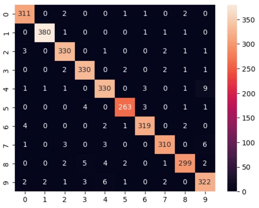
print(clf.score(X_test, y_test)) # 0.9678787878787879
sns.heatmap(confusion_matrix(y_test, clf.predict(X_test)), annot=True, fmt='d')
GaussianNB
from sklearn.naive_bayes import GaussianNB
clf = GaussianNB()

clf.fit(X_train, y_train)
print(clf.score(X_test, y_test)) # 0.8815151515151515

sns.heatmap(confusion_matrix(y_test, clf.predict(X_test)), annot=True, fmt='d')

Conclusion
The RBM is an invaluable asset in any machine learning toolkit, offering a unique combination of power, simplicity, and flexibility. It is a powerful tool for extracting features from datasets, allowing to uncover hidden patterns and relationships. By leveraging the capabilities of RBMs, one can distill complex data down into meaningful insights, and gain a deeper understanding of what drives data. In theory, computing these features isn't easy - in fact, it can be downright computationally expensive. However, by applying clever approximations and parallelization techniques, researchers have been able to significantly speed up the process, making it possible to train RBMs on large datasets in a relatively short amount of time.
While my code may be lacking in terms of parallelization, cleanliness, and separation of concerns - principles that are essential for scalable and maintainable software - it's still worth taking a look at. Think of it as a rough-around-the-edges proof of concept, implemented without the luxury of these best practices. Despite its rough edges, this code can still serve as a valuable starting point for further development and refinement.
I'd be thrilled to receive any feedback on my code, and I'm eager to learn from your insights. As I continue to work on refining my skills, your comments and suggestions could play a huge role in helping me improve my ability to write clean, efficient, and well-structured code. So please, don't hesitate to share your thoughts - your feedback could be just what I need to take my coding abilities to the next level!
Love and peace

References
[1] Upadhya, V., Sastry, P.S. An Overview of Restricted Boltzmann Machines. J Indian Inst Sci 99, 225–236 (2019). https://doi.org/10.1007/s41745-019-0102-z
[2] K. Swersky, D. Tarlow, I. Sutskever. Cardinality Restricted Boltzmann Machines. Dept. of Computer Science, University of Toronto. http://www.cs.toronto.edu/~rsalakhu/papers/CaRBM.pdf
[3] G.E. Hinton. Training products of experts by minimizing contrastive divergence. Neural Computation,
14(8):1771–1800, 2002
[4] Hinton, G. (2010). A Practical Guide to Training Restricted Boltzmann Machines,Version 1. University of Toronto
[5] Keyvanrad, Mohammad & Homayoonpoor, Mahdi. (2014). Deep Belief Network Training Improvement Using Elite Samples Minimizing Free Energy. International Journal of Pattern Recognition and Artificial Intelligence. 29. 10.1142/S0218001415510064.
[6] Carreira-Perpin M. Hinton G. On Contrastive Divergence Learning. University of Toronto.
Supporting
Support my work by renting space on my website: The Link